Rate Graphs and Orders
Quick Notes
- Concentration–Time Graphs
- 0 order: straight line, constant gradient
- 1st order: exponential curve
- Rate = gradient at any point
- Half-Life from Graphs
- First-order reactions have a constant t1/2
- Rate Constant from Half-Life
k = ln(2) / t1/2 - Rate–Concentration Graphs
- 0 order: horizontal line
- 1st order: straight line through origin, k = gradient
- 2nd order: curve
- Investigating Rates
- Methods: initial rates and continuous monitoring
- Use colorimetry for coloured species
Full Notes
See rates and rate equations for essential background theory to this page.
The rate equation cannot be predicted from a balanced chemical equation. It must be determined experimentally, as some reactants may not affect rate.
There are several ways we can determine the orders with respect to each reactant.
Continuous Monitoring Method
We can measure concentration at different times during a reaction. This can be a useful method when it’s difficult to measure initial rates directly.
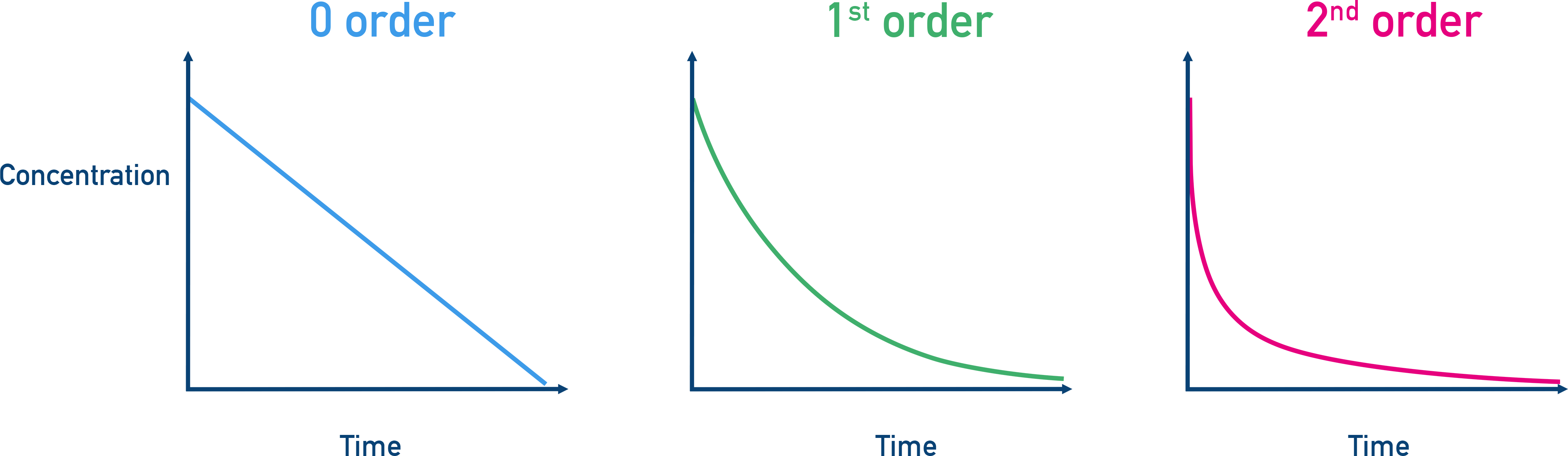
We can use graphs of concentration vs. time to determine the order.
Graphical Interpretation of Orders:
- Zero Order: Concentration vs. time graph is linear (constant rate)
- First Order: Concentration vs. time graph is exponential decay
- Second Order: Concentration vs. time graph is a steeper exponential decay
We can also use concentration–time graphs to find a rate of reaction at any given point by drawing a tangent and finding the gradient.
For example, the initial rate can be determined by drawing a tangent at t=0 and finding the gradient.

Half-Life of First Order Reactions
Half life (t1/2) refers to the time taken for the concentration of a species to halve.
A key feature of a first-order reaction is a constant half-life: The time for concentration to halve is always the same, no matter the starting concentration.
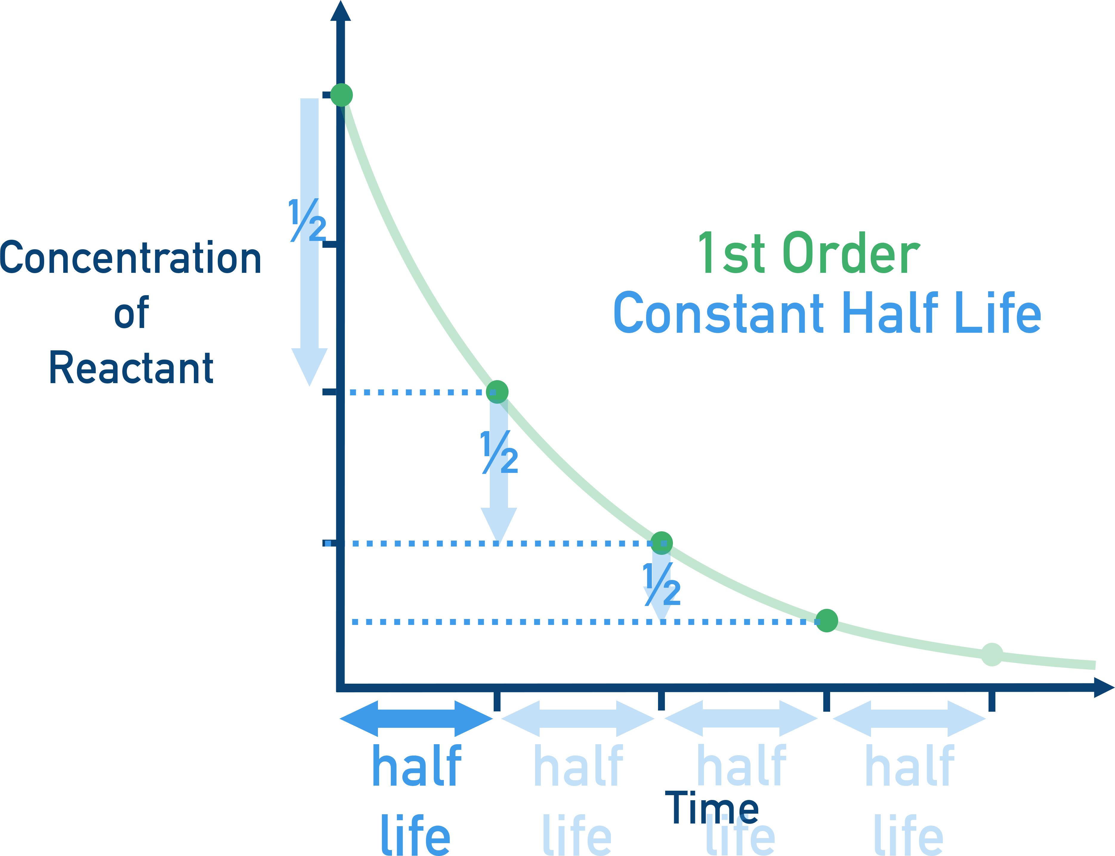
This is useful when confirming that a reaction is first-order.
For first-order reactions: k = ln(2) / t1/2
where t1/2 is the half life (time taken for concentration of reactant to halve).
This is useful when you know the half-life and want to find the rate constant.
Rate–Concentration Graphs
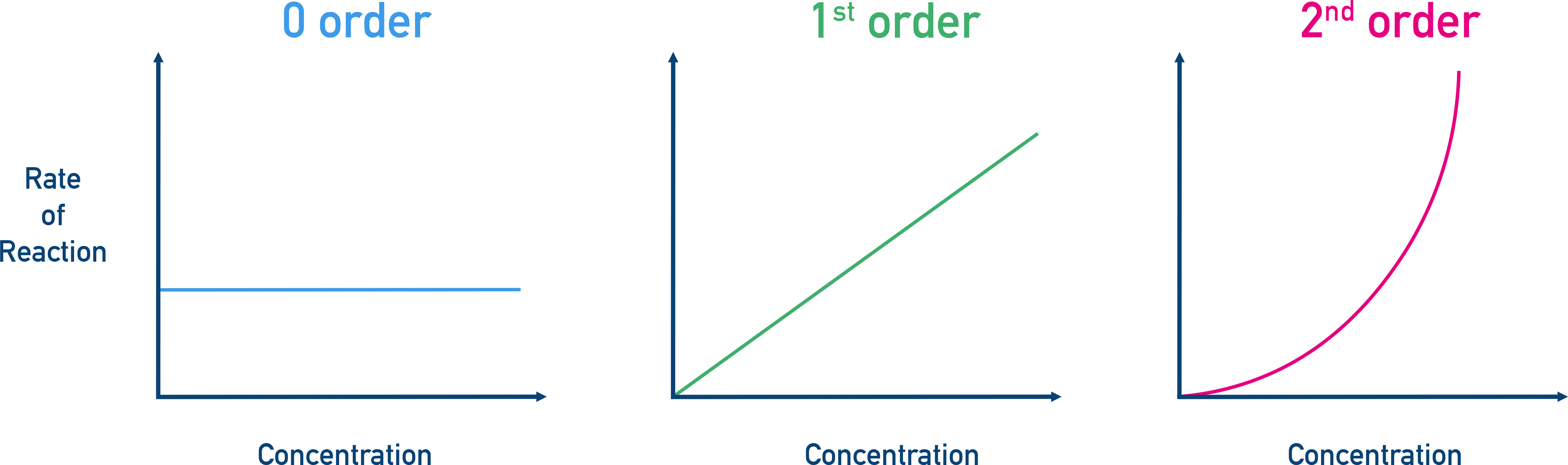
Plotting rate vs concentration shows how the rate changes with concentration of a reactant.
The shape of the graph can be used to determine the order with respect to the reactant.
- Zero Order: Horizontal line (rate is constant)
- First Order: Diagonal straight line through origin (rate ∝ [A])
- Second Order: Upward curve (rate ∝ [A]²)
For first order, the gradient = k.
Experimental Techniques for Measuring Rates
- Initial rates: Vary initial concentrations, measure how quickly a visible change occurs (e.g. time for colour to appear)
- Continuous monitoring: Measure concentration or mass/volume over time
- Colorimetry: Monitor colour intensity for coloured species (e.g. iodine or transition metals)
Determine Orders of Reaction Example
Example: Determining orders from rate data
Reaction: A + B → Products
| exp | [A] (mol dm−3) | [B] (mol dm−3) | Initial Rate (mol dm−3 s−1) |
|---|---|---|---|
| 1 | 0.10 | 0.10 | 0.02 |
| 2 | 0.20 | 0.10 | 0.04 |
| 3 | 0.20 | 0.20 | 0.16 |
[A] has doubled from exp. 1 to exp. 2 and [B] is constant. Rate has doubled (0.02 to 0.04). This means reaction must be first order with respect to A.
[B] has doubled from exp. 1 to exp. 3 and [A] is constant. Rate has quadrupled (x4), gone from 0.04 to 0.16. This means reaction must be second order with respect to B.
Thus, the rate equation is: Rate = k [A]¹ [B]²
Summary
- Orders of reaction are determined experimentally, not from stoichiometry
- Concentration–time graphs show order by shape and can be used to find rate at any time
- First-order reactions have a constant half-life and k = ln(2)/t1/2
- Rate–concentration graphs show 0, 1st and 2nd order by their distinct shapes
- Experimental techniques include initial rates, continuous monitoring and colorimetry