
Introduction to Equilibrium
Quick Notes
- Dynamic equilibrium is when the rate of the forward reaction equals the rate of the backward reaction for a reversible reaction.
- Occurs in a closed system.
- There is no observable change in macroscopic properties (e.g. colour, pressure, concentration).
- The system is dynamic: reactions are still occurring, but at equal and opposite rates.
- Equilibrium can occur in physical changes (e.g. evaporation/condensation) and chemical reactions.
Full Notes
What Is Dynamic Equilibrium?
A system is in dynamic equilibrium when the rate of the forward reaction equals the rate of the reverse reaction.
Dynamic equilibrium can only be reached in a closed system (no matter can enter or leave).
The concentrations of all species remain constant over time, although particles continue to react.
Dynamic refers to the fact that reactions are ongoing, and equilibrium because the system appears unchanged at the macroscopic level.
Physical and Chemical Equilibria
Equilibria can involve either physical changes (like phase changes) or chemical reactions.
In both cases, the forward and reverse processes occur at equal rates, but physical equilibria involve no change in chemical identity, while chemical equilibria involve the making and breaking of chemical bonds, forming new substances in each direction.
ExamplePhysical equilibrium example:
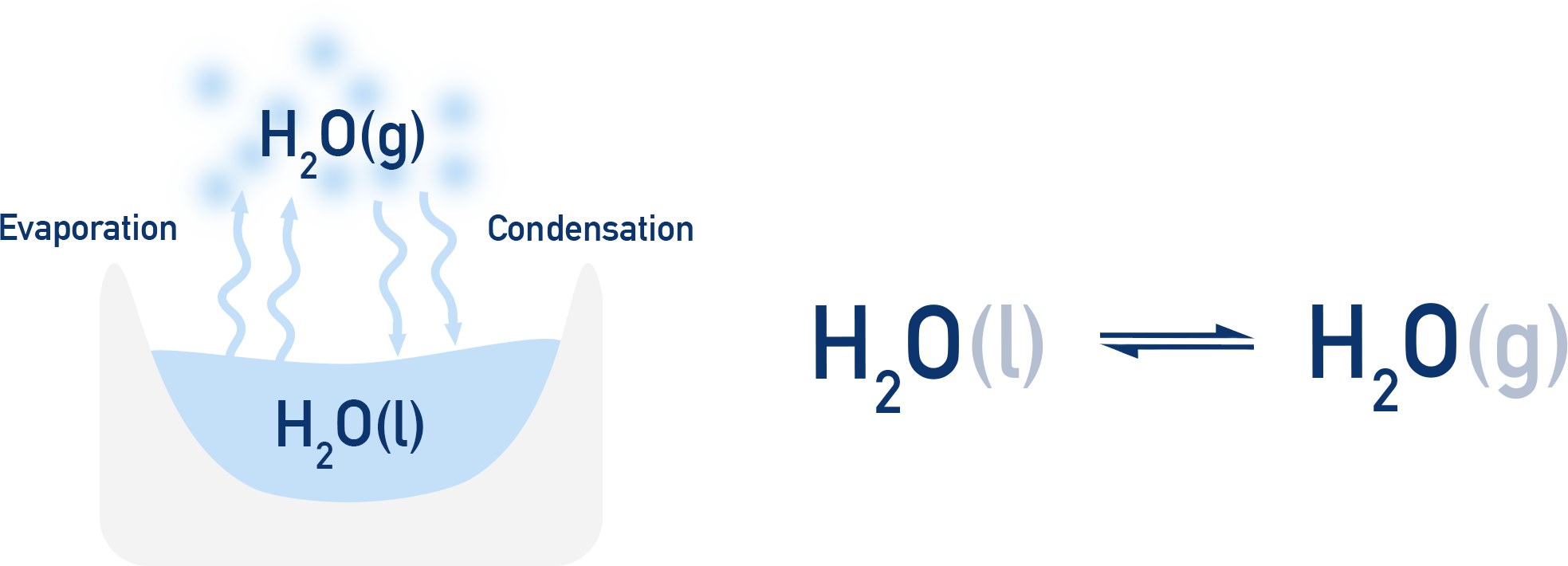
H2O(l) ⇌ H2O(g)
- Water evaporates and condenses at the same rate.
- The amount of liquid and vapour stays constant.
ExampleChemical equilibrium example: The Haber Process (Ammonia Production)

Forward reaction: N2 + H2 → NH3
Reverse reaction: NH3 decomposes into N2 and H2
If the system is left for a short period of time, equilibrium will be reached where the forward reaction occurs at the same rate as the reverse reaction — meaning concentrations of everything remain constant.
Understanding Equilibrium Through Graphs
Graphs can show how a chemical system changes over time as it approaches equilibrium.
Whether we’re looking at concentration, rate of reaction, or partial pressure, the overall pattern is the same: changes at first, followed by a steady state.
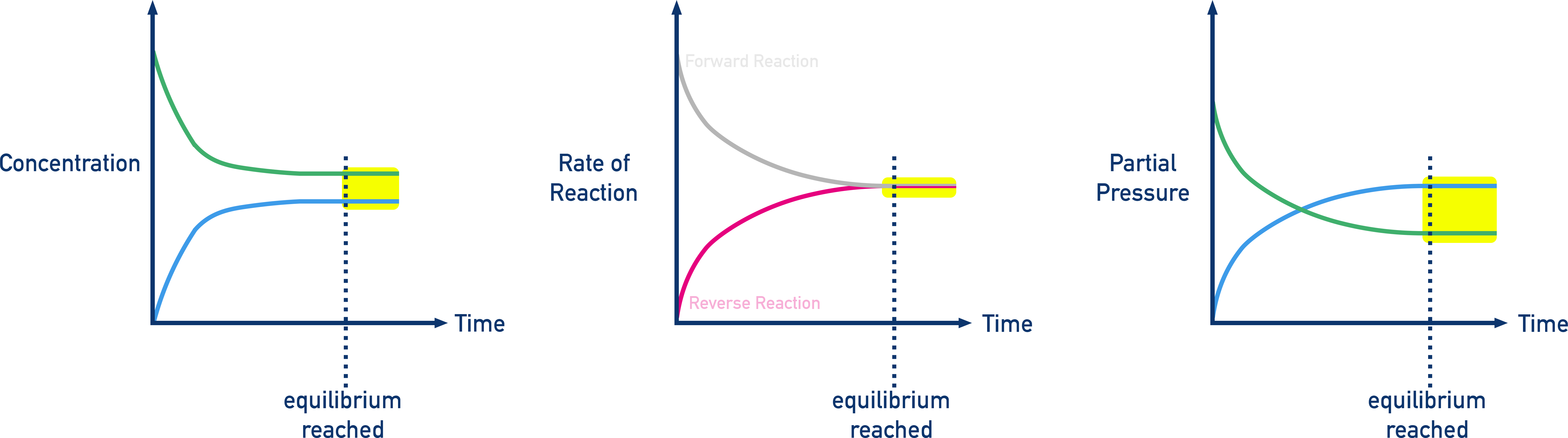
- Concentration vs. Time (Left graph): The concentration of reactants (green) decreases, while the concentration of products (blue) increases. Once equilibrium is reached, both levels flatten — they remain constant, though the reactions are still happening in both directions.
- Rate of Reaction vs. Time (Middle graph): Initially, the forward reaction is faster than the reverse. Over time, the reverse reaction speeds up as more product forms. At equilibrium, both rates become equal, meaning no net change occurs — the system is dynamic, but balanced.
- Partial Pressure vs. Time (Right graph): For gaseous reactions, partial pressures behave just like concentrations. The graph shows reactants’ pressures falling and products’ rising until both level out. This is another way to observe equilibrium being established.
Together, these graphs help illustrate that equilibrium is not when reactions stop, but when they occur at the same rate in both directions, leading to constant observable properties like concentration and pressure.
Key Characteristics of Equilibrium
- Closed system: No exchange of matter with surroundings.
- Forward and reverse reactions: Continuous and occur at equal rates.
- No net change: Concentrations of reactants and products remain constant.
- Macroscopic properties: Pressure, colour, and concentration remain constant.
- Dynamic nature: The system is dynamic, not static.
- Reversibility: Equilibrium can be established from either direction (forward or reverse).